9 Types of Data Distribution in Statistics

Statistical data analysis becomes your competitive advantage when you understand how data points spread across distributed systems and statistical models. Using actual data allows for a more accurate understanding of the spread and patterns of data points, which is crucial for effective statistical analysis in both traditional statistics and modern distributed architectures. It empowers you to go beyond numbers and comprehend the underlying patterns, relationships, and probabilities that drive business decisions. A crucial aspect of statistical analysis involves understanding the different types of data distribution across both mathematical models and distributed computing environments.

By learning how data points spread out, you can analyze data to infer meaningful interpretations and predictions based on the data's shape, central tendency, and variability. This knowledge empowers you to make informed decisions, test hypotheses, and develop models that scale across modern data architectures. A data-distribution service plays a significant role in enhancing data accessibility and processing in statistical analysis, particularly in cloud-native and hybrid environments. But before we discuss any data distribution types, let's understand more about data and how it flows through modern systems.

What Are Data Distributions?

Data distributions are a fundamental concept in statistics and data science that extends beyond traditional mathematical models into modern distributed computing architectures. Analyzing data through the lens of distributions helps in predicting outcomes and understanding various phenomena across both statistical models and real-time data streaming environments. They describe how data points are spread out or clustered around certain values or ranges, whether in a statistical sample or across distributed systems processing petabytes of information daily. Understanding these distributions is crucial for making informed decisions and predictions, as it reveals the data's characteristics and patterns in both historical analysis and real-time processing scenarios.

A discrete probability distribution applies to categorical or discrete variables, where each possible outcome has a non-zero probability, forming the foundation for event-driven architectures and streaming analytics.

There are various types of data distributions, each with unique properties that apply to different contexts. Normal distributions are symmetrical and bell-shaped, ideal for modeling natural phenomena like human height or test scores, as well as network latency patterns in distributed systems. Binomial distributions model the number of successes in a fixed number of independent trials, such as the number of heads in a series of coin flips or successful API calls in microservices architectures. Poisson distributions are useful for modeling the number of events occurring within a fixed interval of time or space, such as customer arrivals at a store or message arrival rates in streaming platforms like Apache Kafka. By understanding these distributions, you can better analyze your data, identify key trends, and make more accurate predictions while designing resilient distributed systems that handle data flow efficiently.

What Are the Different Types of Data?

You can broadly classify data into qualitative and quantitative categories based on its nature, with additional considerations for how data flows through modern distributed architectures. Qualitative data is non-numerical and provides a depth of understanding using descriptive characteristics like color, customer reviews, or system status indicators in monitoring dashboards. Quantitative data, on the other hand, represents data that can be measured or counted, like customer visits per month, ratings between one and five, or throughput metrics in data pipelines processing millions of events per second.

It is crucial to understand the actual distribution of your data rather than assuming it follows a normal distribution, as this can lead to more accurate modeling and predictions in both statistical analysis and distributed system design where data patterns directly impact performance and reliability.

A probability function is used to describe the likelihood of different outcomes for continuous variables, providing a mathematical framework for data analysis that extends to real-time decision making in streaming architectures and edge computing environments.

Quantitative data is particularly relevant to data-distribution analysis, and you can further classify it as discrete and continuous data, with modern applications spanning from traditional statistical models to distributed data processing frameworks.

Discrete Data

This type of data consists of distinct, separate values that appear in both statistical sampling and event-driven systems. A discrete distribution represents the probabilities of distinct outcomes, such as the number of students in a class or the count of successful message deliveries in distributed messaging systems. The probability mass function (PMF) is a mathematical function that describes the probabilities of discrete outcomes, serving as the foundation for designing resilient data pipelines and understanding system behavior patterns. It often represents whole numbers or counts, such as the number of students in a class, the number of heads in 10 coin flips, or the number of concurrent connections to a database cluster, with a finite number of possible values. You can represent discrete data using bar charts, histograms, or real-time dashboards that monitor discrete events across distributed systems.

Continuous Data

Contrarily, continuous data can take on any value within a given range—for example, height, weight, time, or system latency measurements in distributed architectures. A continuous random variable can take on an infinite number of values within a given range, making it essential for modeling phenomena like response times, bandwidth utilization, and resource consumption in cloud-native environments.

In contrast, a discrete uniform distribution is a type of distribution where all outcomes are equally likely, such as rolling a six-sided die or load balancing requests across identical server instances. You can measure these values to any degree of precision within the relevant range and represent them using line graphs, density plots, or real-time monitoring visualizations that track continuous metrics across distributed infrastructure. A bivariate distribution is particularly useful in analyzing relationships between two continuous variables, such as height and weight, or CPU utilization and memory consumption in containerized applications, providing insights into their interactions and system optimization opportunities.

Understanding whether your data is discrete or continuous is crucial for choosing the appropriate data-distribution model for analysis and designing efficient data processing architectures that scale with business growth.

What Are the Key Characteristics of Continuous Data?

Continuous-data distributions measure data points over a range rather than as individual points, applying to both traditional statistical analysis and modern distributed system metrics like throughput, latency, and resource utilization patterns. Continuous probability distributions model and interpret continuous variables, encompassing infinite values within a range, making them essential for understanding system behavior in cloud-native architectures where performance metrics vary continuously. The expected value, or mean, of a distribution is crucial for understanding the outcomes of random variables in statistical scenarios and for setting baseline performance expectations in distributed systems monitoring.

Often measured on a scale, such as temperature, weight, or system response time, continuous data can be represented using a histogram, probability-density function, or real-time monitoring dashboards that display continuous metrics across distributed infrastructure. The normal distribution, or Gaussian distribution, is a common type of continuous distribution that is symmetric about the mean, forming a bell-shaped curve that frequently appears in network latency measurements, user behavior patterns, and resource consumption metrics in well-designed distributed systems.

Other continuous distributions include the exponential distribution, which models the time between events in a Poisson process and is fundamental for understanding inter-arrival times in message queues and streaming platforms. The gamma distribution can handle skewed data commonly found in system performance metrics, while the log-normal distribution is useful for data that grows multiplicatively, such as data volume growth in analytics pipelines. Recognizing these characteristics is crucial for selecting the right statistical analysis techniques and designing monitoring systems that accurately capture the behavior of distributed architectures.

What Is Probability Distribution?

A probability distribution is a mathematical function that assigns a probability to each possible value or outcome of a random variable, forming the theoretical foundation for both statistical analysis and practical applications in distributed systems design. It describes the likelihood of different events or outcomes, providing a framework for predicting and analyzing data behavior in contexts ranging from traditional hypothesis testing to real-time decision making in streaming data architectures. Probability distributions can be discrete—such as the binomial distribution modeling successful API calls or Poisson distribution describing message arrival rates in event-driven systems—or continuous—such as the normal distribution characterizing response times or exponential distribution modeling failure intervals in distributed infrastructure.

The probability-density function (PDF) describes the probability of different values or outcomes, while the cumulative distribution function (CDF) describes the probability that a random variable takes on a value less than or equal to a given value, both critical for understanding system behavior and setting appropriate thresholds in monitoring and alerting systems. Understanding probability distributions is crucial for statistical analysis, hypothesis testing, decision-making, and designing resilient distributed systems that can handle variability in data patterns, user behavior, and system performance while maintaining reliability and performance standards.

How Do You Define Data Distribution?

Data distribution refers to how data spreads across a range of values, encompassing both statistical distributions in mathematical models and physical data distribution across distributed computing infrastructure. The center value plays a crucial role in understanding how data clusters around a particular value, helping to interpret the skewness and symmetry of the distribution while also informing load balancing and data partitioning strategies in distributed systems. It describes the arrangement of your data, whether it clusters around a particular value, is scattered evenly, or skews in one direction, with implications for both statistical inference and system architecture decisions that affect performance and scalability.

Data distribution also provides insights into the frequency or probability of specific outcomes, which translates directly to understanding traffic patterns, resource utilization, and failure modes in distributed architectures where data flows across multiple nodes, geographic regions, and processing layers. In statistics, based on the type of quantitative data, there are two fundamental types of data distribution—discrete and continuous—while in distributed systems, data distribution strategies include replication, sharding, and streaming patterns that ensure availability, performance, and consistency across diverse computing environments.

What Are the Most Common Methods to Analyze Distribution of Data in Statistics?

Understanding the methods to analyze distribution of data in statistics is fundamental for effective data analysis, spanning from traditional statistical inference to modern distributed system monitoring and optimization. Modern statistical analysis employs various sophisticated techniques that go beyond simple visual inspection to provide rigorous, quantitative assessments of data distribution patterns, with applications extending to real-time analytics and distributed system performance analysis.

Goodness-of-Fit Testing Approaches

Kolmogorov-Smirnov test compares your sample distribution to a theoretical distribution, measuring the maximum distance between cumulative distribution functions, making it valuable for validating assumptions in both statistical models and system performance baselines. Anderson-Darling test offers enhanced sensitivity to deviations in the distribution tails, making it superior for detecting departures from normality in the extremes of your data, particularly useful for identifying outliers in system metrics that could indicate performance issues or security threats. Chi-square goodness-of-fit test works with categorical or grouped continuous data, comparing observed frequencies to expected frequencies under a hypothesized distribution, essential for validating load balancing effectiveness and traffic distribution patterns in distributed architectures.

Automated Distribution Identification Techniques

Automated approaches combine multiple goodness-of-fit statistics to rank distributions by their fit quality, often using information criteria like AIC (Akaike Information Criterion) or BIC (Bayesian Information Criterion) to balance goodness-of-fit against model complexity, enabling data teams to rapidly identify appropriate models for both historical analysis and predictive system monitoring. Machine-learning algorithms can analyze data characteristics including skewness, kurtosis, and tail behavior to recommend appropriate distribution families, supporting automated anomaly detection and adaptive system tuning in cloud-native environments where manual analysis becomes impractical at scale.

Parameter Estimation Methods

Maximum likelihood estimation (MLE) provides asymptotically optimal parameter estimates, forming the backbone of statistical inference and enabling precise modeling of system behavior patterns for capacity planning and performance optimization. Method-of-moments estimation offers computational advantages when closed-form solutions exist, particularly valuable in real-time analytics where computational efficiency directly impacts system responsiveness. Bayesian estimation produces posterior distributions for parameters, delivering uncertainty quantification especially valuable with small samples, supporting risk-aware decision making in distributed system design where uncertainty bounds inform redundancy and failover strategies. Robust estimation techniques such as M-estimators address challenges with outliers and heavy-tailed data commonly encountered in distributed systems where extreme values may indicate system stress, attacks, or configuration issues requiring immediate attention.

What Are the Advanced Distribution Modeling Techniques in Modern Statistics?

Heavy-Tailed Distribution Analysis

Power-law (Pareto, Zipf) distributions and extreme value theory (Gumbel, Fréchet, Weibull) model phenomena where extreme values occur more frequently than a normal distribution predicts, essential for modeling network traffic bursts, data hotspots in sharded databases, and cascading failure patterns in distributed systems where rare events can have disproportionate impact on overall system stability.

Mixture Distribution Modeling

Gaussian mixture models and other finite mixture models combine multiple component distributions to capture multimodal data commonly found in user behavior patterns, system performance profiles, and workload characteristics across different time periods or user segments. The Expectation-Maximization (EM) algorithm is commonly used for parameter estimation, enabling automated identification of distinct operational modes in distributed systems where performance characteristics may vary significantly based on load patterns, geographic distribution, or application types.

Copula-Based Modeling

Copulas separate marginal distributions from dependence structures, enabling flexible multivariate modeling essential for understanding correlations between different system metrics like CPU utilization and memory consumption, or between business metrics and infrastructure performance. Archimedean copulas (Clayton, Gumbel, Frank) and vine copulas handle complex dependency patterns in higher dimensions, supporting sophisticated monitoring and alerting systems that consider multiple correlated metrics rather than treating each metric independently, reducing false positives and improving incident response effectiveness.

How Do Data Distribution Principles Apply to Modern Distributed Systems and Architectures?

The evolution from monolithic data processing to distributed architectures has transformed how organizations think about data distribution, extending statistical concepts into practical system design patterns that handle petabytes of data across global infrastructure. Modern data distribution strategies leverage both mathematical distribution principles and distributed computing patterns to create resilient, scalable systems that maintain performance under varying load conditions while ensuring data consistency and availability across multiple nodes and geographic regions.

Event-Driven Architectures and Statistical Patterns

Decoupling components through domain-driven decomposition separates producers from consumers via brokers like Apache Pulsar, which handles 100,000+ consumers per topic while applying Poisson distribution principles to model message arrival rates and optimize buffer sizes. This prevents cascading failures when downstream processors fail, with statistical models helping predict queue depths and automatically scale consumer groups based on traffic patterns. Load balancing algorithms use exponential distribution models to predict failure intervals and implement circuit breaker patterns that protect system stability during peak traffic periods.

Message delivery semantics require understanding of probability distributions to optimize system behavior. At-least-once delivery suits payment transactions requiring guaranteed execution, where binomial distribution models help calculate retry probabilities and optimize acknowledgment timeouts. Exactly-once semantics via Kafka's transactional API prevents duplicate processing in financial reconciliations, using statistical analysis to balance throughput overhead against consistency guarantees, typically adding 15% processing overhead versus at-least-once delivery patterns.

Monitoring and error handling leverage statistical distribution analysis through cross-silo logging with OpenTelemetry traces that track event journeys across clouds. Anomaly detection algorithms trigger automated rollbacks when data drift exceeds three-sigma thresholds, using normal distribution assumptions to identify outliers that may indicate system compromise or configuration errors requiring immediate intervention.

Streaming Platforms and Distribution Optimization

Apache Kafka scaling optimization uses statistical models to implement dynamic partition rebalancing via machine learning algorithms that redistribute load during traffic spikes without downtime. Consistent hashing principles from probability theory ensure uniform data distribution across partitions, while statistical analysis of consumer lag patterns enables predictive scaling that maintains sub-second processing latencies even during traffic surges exceeding normal distribution boundaries.

Apache Pulsar's segment-centric architecture outperforms traditional approaches in multi-tenant scenarios by isolating traffic per namespace using probability-based routing algorithms. Statistical analysis of tenant behavior patterns enables automated resource allocation that processes 100+ billion daily messages with 99.999% availability, leveraging gamma distribution models to predict resource requirements and optimize storage tier placement based on access patterns and retention requirements.

Real-time data processing applies distribution principles to optimize window operations, watermarking strategies, and late-arriving data handling. Streaming systems use exponential distribution models to predict processing delays and automatically adjust window boundaries, while Weibull distribution analysis helps optimize checkpoint intervals and failure recovery procedures, ensuring system resilience during traffic spikes or partial system failures.

What Are the Essential Data Replication and Distribution Strategies for Modern Infrastructure?

Contemporary data infrastructure requires sophisticated replication and distribution strategies that combine traditional database principles with cloud-native architectures, ensuring data availability, consistency, and performance across geographically distributed systems while maintaining cost efficiency and regulatory compliance. These strategies apply statistical distribution principles to optimize placement, replication factors, and synchronization patterns based on access patterns, failure probabilities, and business requirements.

Advanced Replication Techniques and Trade-offs

Synchronous versus asynchronous replication requires understanding statistical trade-offs between consistency, latency, and availability. Synchronous replication guarantees immediate consistency across nodes but introduces latency typically ranging from 15-50 milliseconds depending on geographic distribution, making it essential for financial transactions where data integrity outweighs performance considerations. Asynchronous replication provides sub-second response times with eventual consistency, suitable for social media activity feeds where slight delays are acceptable in exchange for global scalability and performance.

Change Data Capture (CDC) implementation via tools like Debezium streams database write-ahead logs to message brokers like Kafka, enabling warehouse synchronization within 500 milliseconds while maintaining exactly-once delivery guarantees. Statistical analysis of CDC lag patterns helps optimize buffer sizes and batch intervals, with automated scaling algorithms that adjust replication throughput based on source system activity patterns and downstream processing capacity.

Snapshot-based replication provides point-in-time consistency for compliance and backup scenarios, using statistical sampling techniques to optimize snapshot intervals based on data change velocities and recovery time objectives. Incremental snapshot strategies leverage delta compression and deduplication algorithms to minimize storage and bandwidth requirements, with probability-based scheduling that distributes snapshot operations to minimize impact on production workloads.

Database Sharding and Distributed Data Management

Consistent hashing for key-based sharding distributes data across multiple database nodes using hash functions that ensure uniform distribution while minimizing data movement during scaling operations. Statistical analysis of key distribution patterns helps identify potential hotspots before they impact performance, with automated rebalancing algorithms that redistribute shards when partition skew exceeds acceptable thresholds, typically 25% variance from expected distribution patterns.

Geographic sharding strategies leverage statistical analysis of user behavior patterns and access frequencies to optimize data placement across global regions. Data locality optimization places frequently accessed data closer to users while maintaining compliance with data sovereignty regulations, using predictive models based on user behavior patterns to pre-position data and reduce cross-region bandwidth costs by up to 60%.

Multi-dimensional sharding combines multiple distribution strategies like time-based partitioning for temporal data, geographic partitioning for user data, and hash-based partitioning for uniform distribution. Statistical models help optimize partition boundaries and replication factors based on query patterns, data growth rates, and performance requirements, ensuring consistent performance as data volumes scale from gigabytes to petabytes while maintaining query response times within acceptable service level agreements.

What Are the Different Types of Data Distribution in Statistics?

Data distributions provide mathematical models that describe the behavior of random variables across both traditional statistical analysis and modern distributed computing environments. By identifying the type of distribution that fits the data—such as Poisson for message arrival rates, Binomial for success/failure scenarios, or Gaussian for performance metrics—you can estimate parameters that best define your data distribution and use them to simulate new data points, optimize system performance, and predict behavior patterns in distributed architectures.

Discrete Distributions

Bernoulli Distribution

The Bernoulli distribution describes the probability of a single event with binary results such as success (1) or failure (0), fundamental for modeling binary outcomes in both statistical analysis and distributed systems. Typical applications include binary-classification problems, click-through rate prediction, churn-rate analysis, and system health monitoring where services are either available or unavailable. In distributed architectures, Bernoulli distributions model node availability, API call success rates, and circuit breaker states, providing the foundation for reliability engineering and automated failover decision-making processes.

Binomial Distribution

Models the probability of getting a specific number of successes in a fixed number of independent trials, essential for analyzing batch processing outcomes, distributed task completion rates, and quality assurance testing where you need to understand the distribution of successful operations out of a known number of attempts. In modern data infrastructure, binomial distributions help optimize batch sizes, predict processing success rates, and design retry mechanisms that balance throughput with error recovery capabilities.

Poisson Distribution

Approximates the number of events occurring in a fixed interval given an average rate λ (lambda), fundamental for modeling message arrival rates in streaming platforms, user behavior patterns, and system failure events. In distributed systems, Poisson distributions help size message queues, predict traffic spikes, and optimize consumer group configurations in platforms like Apache Kafka where message arrival patterns directly impact processing efficiency and system stability.

For numerical evaluation, try this Poisson distribution calculator.

Geometric Distribution

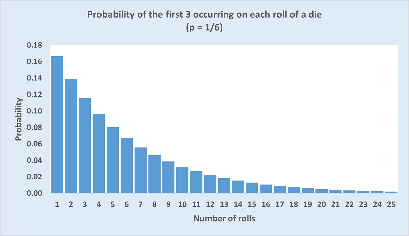
Models the probability of the number of failures before the first success in a series of independent trials, valuable for analyzing retry mechanisms, connection establishment patterns, and recovery procedures in distributed systems. This distribution helps optimize exponential backoff strategies, circuit breaker thresholds, and failure recovery policies by providing statistical frameworks for understanding how many attempts typically occur before successful operations, enabling systems to balance persistence with resource efficiency.

Continuous Distributions

Normal Distribution

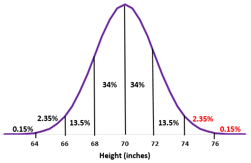
Represents symmetrical data around a central mean with the characteristic bell curve, commonly observed in system response times, resource utilization patterns, and user behavior metrics in well-designed distributed systems. Normal distributions provide the foundation for statistical process control, anomaly detection algorithms, and capacity planning models that use standard deviation boundaries to identify outliers and predict system behavior under varying load conditions.

F Distribution

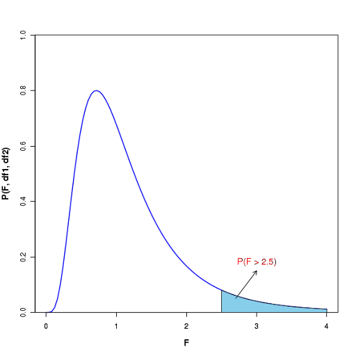
Arises when comparing variances of two normally distributed populations, particularly valuable for A/B testing scenarios, performance comparison between different system configurations, and ANOVA-based analysis of variance in distributed system performance metrics. F distributions help determine whether observed performance differences between systems, algorithms, or configurations are statistically significant, supporting data-driven decision making in system optimization and architecture selection processes.

Chi-Square Distribution

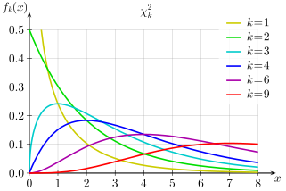
Used in tests of independence and goodness-of-fit, essential for validating assumptions about data relationships, testing load balancing effectiveness, and analyzing categorical data patterns in user behavior and system usage statistics. Chi-square distributions support hypothesis testing in distributed systems where you need to validate whether observed traffic patterns, error rates, or resource utilization align with expected distributions, enabling evidence-based system tuning and capacity planning decisions.

Exponential Distribution

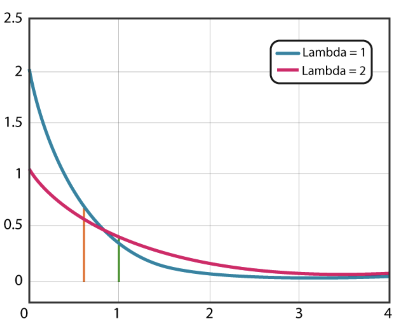
Models the time between events in a Poisson process and is notable for its memoryless property, making it fundamental for modeling inter-arrival times in message queues, failure intervals in distributed systems, and service time distributions in queuing theory applications. The memoryless property makes exponential distributions particularly valuable for modeling system failures and recovery procedures where past events don't influence future probabilities, supporting robust reliability engineering and automated failure recovery mechanisms.

Gamma Distribution

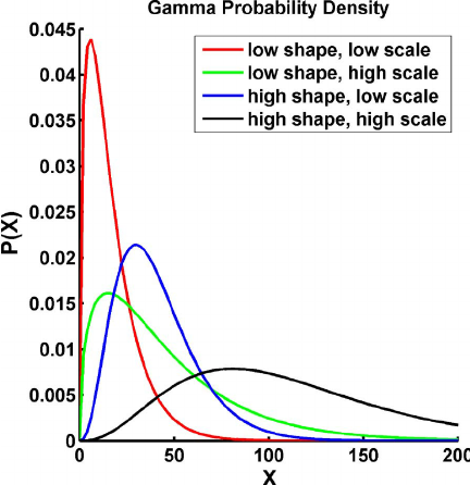
Characterized by a shape (α) and scale (β) or rate (λ) parameter, ideal for modeling positively skewed data commonly found in system performance metrics, processing times, and resource consumption patterns that exhibit right-tail behavior. Gamma distributions excel at modeling cumulative processes like total processing time for batch jobs, aggregate resource consumption over time periods, and service level agreement compliance analysis where performance metrics naturally exhibit positive skewness due to occasional high-impact outliers.

How Do You Effectively Visualize Data Distributions?

Probability-mass functions (PMFs) visualize discrete-outcome probabilities, essential for displaying message success rates, system state distributions, and categorical performance metrics in distributed system dashboards that help operators understand system behavior patterns and identify optimization opportunities. Histograms show the distribution of continuous variables like response times, resource utilization, and throughput metrics, enabling rapid identification of performance anomalies and capacity planning insights through visual pattern recognition.

Box plots summarize central tendency, variability, and outliers in system metrics, providing compact visualizations perfect for comparing performance across different system configurations, time periods, or geographic regions while highlighting potential issues requiring investigation. Scatter plots reveal relationships between two variables such as CPU utilization versus memory consumption, request rate versus response time, or user activity versus system load, enabling correlation analysis that supports system optimization and capacity planning decisions.

Standard deviation measures variability around the mean, providing quick insight into data spread and potential outliers that may indicate system stress, configuration issues, or security threats requiring immediate attention. Effective visualizations make it easier to convey complex statistical insights to both technical and non-technical stakeholders, supporting data-driven decision making across development teams, operations staff, and business leadership while maintaining the statistical rigor necessary for reliable system management and optimization.

FAQs

1. Why is understanding data distribution important in distributed systems?

‍It helps teams predict system behavior, optimize resources, and avoid performance issues. Distributions like Poisson or Gamma model real-world patterns like message spikes or resource usage, enabling smarter scaling and more reliable system design.

2. How do discrete and continuous distributions apply to monitoring?

‍Discrete distributions track counts (e.g., API calls), while continuous ones measure ranges (e.g., latency). Using both helps monitoring tools detect anomalies, set thresholds, and improve system reliability.

3. Can machine learning improve distribution modeling?

‍Yes—ML can detect patterns, skew, and anomalies in large datasets automatically. It enables real-time distribution analysis and adaptive system tuning at scale.

4. What’s the difference between probability and physical data distribution?

‍Probability distribution models outcomes statistically (like latency), while physical distribution refers to how data is stored or processed across systems (like sharding). Both influence performance and reliability.

‍