4 ways to optimize your BigQuery tables for faster queries

BigQuery is a popular analytical database (OLAP) on the Google Cloud Platform. It’s designed (and optimized) for heavy analytical queries on datasets Terabytes and Petabytes large. It differs from OLTP databases such as Postgres, which are optimized for CRUD (create, read, update, delete) operations.

As powerful as BigQuery is, it’s essential to design your BigQuery tables and write SQL queries that are efficient, giving you the correct results in the fastest and most cost-effective way. This is rarely a problem when dealing with small datasets, but as you scale, poorly written queries and inadequate architectures start to stick out like a sore thumb.

BigQuery separates the storage and compute components which allows for independent scaling of both. In this article, we explore design patterns of your BigQuery storage that you can use to increase speed and performance of your queries. We’ll cover strategies for optimizing your SQL queries in a later article.

Understanding BigQuery storage costs

BigQuery provides managed distributed storage. Data can be stored in tables, materialized views, external tables and table snapshots. Data in BigQuery is stored column-wise, i.e., columns are stored together, which makes it very powerful for running analytical queries.

When you run <span class="text-style-code">SELECT COUNT(id) FROM sales</span>, BigQuery can run this in a very short time as it needs to read only one column, and not multiple rows of data. On the flip side, running <span class="text-style-code">SELECT id FROM sales WHERE status = 'closed'</span> means traversing multiple columns, combining the data into rows then returning an output… obviously a slower operation.

BigQuery charges for the data stored based on whether active i.e. modified in the last 90 days or inactive i.e. not modified in the last 90 consecutive days. This ranges between $0.02/GB - $0.04GB for active and $0.01/GB - $0.02/GB with the first 10GB per month free.

Understanding BigQuery compute costs

Whenever you run a query against your data, BigQuery creates (in parallel), schedules, and runs workers that transfer data from the storage cluster via a high-speed network, run the query (in memory), and return results.

The compute cluster processes/scans an amount of data defined by your query, with more data processed as you select more columns. The size of data is dependent on the columns’ data types, ranging from 1 logical byte (Boolean) to 32+ logical bytes (Bignumeric).

It’s important to note that BigQuery charges you for the amount of data scanned (with 1TB free per month) and not the data output. BigQuery doesn’t yet charge for data transferred over the network between the storage and compute clusters.

How to investigate BigQuery performance issues

BigQuery offers two visual tools to identify bottlenecks to your query’s performance quickly. These show how much data the query is expected to process and the steps taken in the query execution.

Look at the amount of data to be processed before running the query

For queries written on the BigQuery console, the amount of data the query will scan when executed is always shown for syntactically correct queries. As explained above, the more data you scan, the more costs you rack up and the slower your query runs.

More often than not, looking at the amount of data to be processed is a straightforward but powerful point to start in your optimization journey. To showcase this, let’s look at two queries that get data from Google’s publicly available dataset on patents.

This query returns all columns from the entire dataset. At the top right of the query editor, we see that the query will process 379.24GB of data.

 If we run the same query but only return two columns, the amount of data to be processed reduces by 99% to 3.43GB!

Use the query plan to understand your query performance

Similar to the EXPLAIN keyword in databases such as Postgres, for each query that you run, BigQuery provides diagnostic information showing the steps taken to execute the query, how long each step took, and compute resources consumed.

Investigating the stages for the different metrics, you may find opportunities for optimization. You can’t necessarily change how execution is done, but you can see areas to improve in your query. 

To illustrate, the query with the plan shown above has a stage that took 793ms of compute (relatively very high compared to the other stages).

We can see this stage runs a JOIN operation that’s reading a large number of records. See that the read time is also relatively high. With this information, we can reduce the number of records to be joined, reducing the read and compute times!

BigQuery recently introduced Execution Graph, a graphical view of the query plan.

4 ways to optimize your storage

Before you even start writing your query, there are steps you can take when designing your Data Warehouse to ensure data is already stored in the most optimal way.

BigQuery does full table and column scans for any given query. In typical OLTP databases, this can be mitigated by indexing columns, which isn’t supported in BigQuery.

In a typical OLTP, you can limit the amount of data scanned by using the keyword LIMIT. Let’s see if that’s the case on BigQuery.

Notice that both these queries will scan 379.24GB when run.

Therefore, it’s very important that your query limits the amount of data being scanned in the first place. At the design stage, you can partition and cluster your tables.

Partition your tables

Partitioning splits your table into smaller logical sections based on a given field. More often than not, date and timestamp columns in the data are used for partitioning. The time of ingestion into BigQuery and integer columns can also be used.

BigQuery manages writing data into partitions by automatically writing new data into the specific partition based on data in the partition column.

When you run a query against a partitioned table, you pass a condition that filters on the partition field. BigQuery will then only scan data in the partition with that value, a process called pruning.

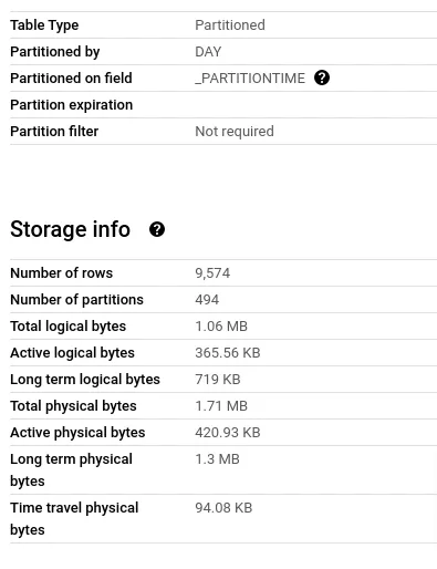
Here is an example of a table partitioned on the field _PARTITIONTIME:

On the BigQuery console, in the table creation UI, you can specify how you want the table partitioned, and for extra safety, whether any queries on that table must have a WHERE clause.

You can tell a table is partitioned on the BigQuery console either by looking at the icon, a banner in the table information, or a section in the table details

Cluster your tables

Clustering orders the contents of your table or partition based on defined columns. The ordered contents are then stored in blocks of correlated values, with data in each block lying between a range of values.

Clustering is quite similar to indexing in OLTP databases. BigQuery keeps track of the start and end of each block similar to a key in an index. This is very useful, especially for columns that you will frequently filter on.  When a query filters on a clustered column, BigQuery will only scan blocks matching the filter.

Clustering has a few of gotchas to note:

• Only Google Standard SQL can query clustered tables
• It’s useful for tables 1GB or more in size
• The cost estimator isn’t as accurate for clustered tables
• When filtering a table clustered on multiple columns you need to include at least the first cluster column in your filter
• When filtering a table clustered on multiple columns the filter order must match the cluster order

Pre-transform your data into materialized views

A view is not a table. It’s a query that’s run every time it’s referenced. Every time you run a query that references a view, the view reference is replaced by the SQL that forms the view.

If you have a view successful_transactions that returns a subset of transactions defined as <span class="text-style-code">SELECT * FROM transactions WHERE status = 'success'</span> then you write a query like <span class="text-style-code">SELECT * FROM successful_transactions sf LEFT JOIN users u ON sf.user_id = u.id</span> what actually runs is:

SELECT *
FROM (
 SELECT *
 FROM transactions
 WHERE status = 'success'
) sf
LEFT JOIN users u ON sf.user_id = u.id

Above, you may have expected that the view would have a reduced amount of data, but what actually happens is that you scan the entire transactions table, filter it, then join data every time you run the query. Note that a query can reference a maximum of 16 views directly or indirectly.

Materialized views are a periodically updated cache of results of the view. These are queried similarly to a normal table which avoids the repeated complete scans and computation of the underlying tables. BigQuery fully manages these to stay up to date about the underlying tables.

You can take advantage of materialized views to store pre-transformed data to be read by other queries i.e. filtering, joining, sorting etc.

You can create materialized views as follows:

CREATE MATERIALIZED VIEW project.dataset.view_name AS (
 -- View definition in the brackets
)

Denormalize your data

In a classic database schema, data is usually normalized with up to 6 normal forms existing. This is okay for OLTP use cases but leads to degraded performance for analytical queries, especially for tables 10GB and up. BigQuery doesn’t even have support for referential integrity via foreign keys!

Denormalization means that you only create a few wide tables with all the needed data, also known as OBT (One Big Table). BigQuery offers data types to make denormalization easier.

STRUCT/RECORD

A row of data (record) can be stored in a column of a table in its completeness and accessed very similarly to JSON data.

ARRAY

Multiple records can be stored in a single column and accessed using the common array indexing methods. To illustrate this, say we have users that can transact on our platform. Classically, we would have two tables: users and transactions with the transactions table having a foreign key referencing a primary key in the users table

If we want the total amount of transactions per user, we would most likely write a query like:

SELECT
 u.id,
 SUM(t.amount) AS total_amount_transacted
FROM transactions t
LEFT JOIN users u ON t.user_id = u.id

If we denormalise our data into one table with user information and a column with all transactions as an ARRAY of RECORDs, we can just do:

SELECT user_id, SUM(tx.amount) AS am
FROM user_info_and_tx,UNNEST(transactions) AS txGROUP BY 1

Conclusion

BigQuery is a petabyte-scale analytics DB utilizing parallel processing to achieve fast querying of massive datasets. To optimize your workloads on BigQuery, you can optimize your storage by:

1. Partitioning your tables
2. Clustering your tables
3. Pre-aggregating your data into materialized views
4. Denormalizing your data

You can also optimize your queries to run faster. We will cover strategies for query optimization in part 2 of this article.